Vegetation Index Analysis with geospatialsuite

Introduction

This vignette demonstrates comprehensive vegetation analysis using geospatialsuite’s 60+ vegetation indices. Learn to monitor plant health, detect stress, and analyze agricultural productivity.

Loading Required Packages

library(geospatialsuite)
library(terra)

Quick Start with Sample Data

# Load sample spectral bands
red <- load_sample_data("sample_red.rds")
nir <- load_sample_data("sample_nir.rds")
blue <- load_sample_data("sample_blue.rds")

# Calculate NDVI using geospatialsuite
ndvi <- calculate_vegetation_index(
  red = red,
  nir = nir,
  index_type = "NDVI"
)

# Visualize
plot(ndvi, main = "Normalized Difference Vegetation Index (NDVI)",
     col = terrain.colors(100))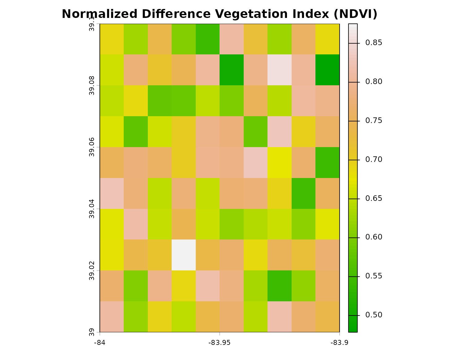

Understanding Vegetation Indices

Common Vegetation Indices

NDVI (Normalized Difference Vegetation Index)

# Calculate NDVI with geospatialsuite
ndvi <- calculate_vegetation_index(
  red = red,
  nir = nir,
  index_type = "NDVI"
)

# Summary statistics
summary(values(ndvi))
#>       NDVI       
#>  Min.   :0.4785  
#>  1st Qu.:0.6473  
#>  Median :0.7172  
#>  Mean   :0.7069  
#>  3rd Qu.:0.7725  
#>  Max.   :0.8752

# Classify vegetation density
vegetation_classes <- classify(ndvi,
  rcl = matrix(c(-Inf, 0.2, 1,
                 0.2, 0.6, 2,
                 0.6, Inf, 3), 
               ncol = 3, byrow = TRUE)
)

plot(vegetation_classes, 
     main = "Vegetation Density Classes",
     col = c("brown", "yellow", "darkgreen"),
     legend = FALSE)
legend("topright", 
       legend = c("Sparse", "Moderate", "Dense"),
       fill = c("brown", "yellow", "darkgreen"))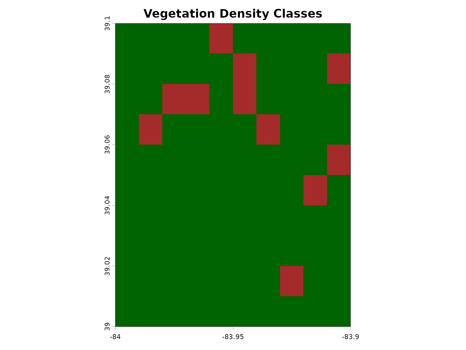

EVI (Enhanced Vegetation Index)

# Calculate EVI using geospatialsuite
evi <- calculate_vegetation_index(
  red = red,
  nir = nir,
  blue = blue,
  index_type = "EVI"
)

# Compare NDVI and EVI
par(mfrow = c(1, 2))
plot(ndvi, main = "NDVI", col = terrain.colors(100))
plot(evi, main = "EVI", col = terrain.colors(100))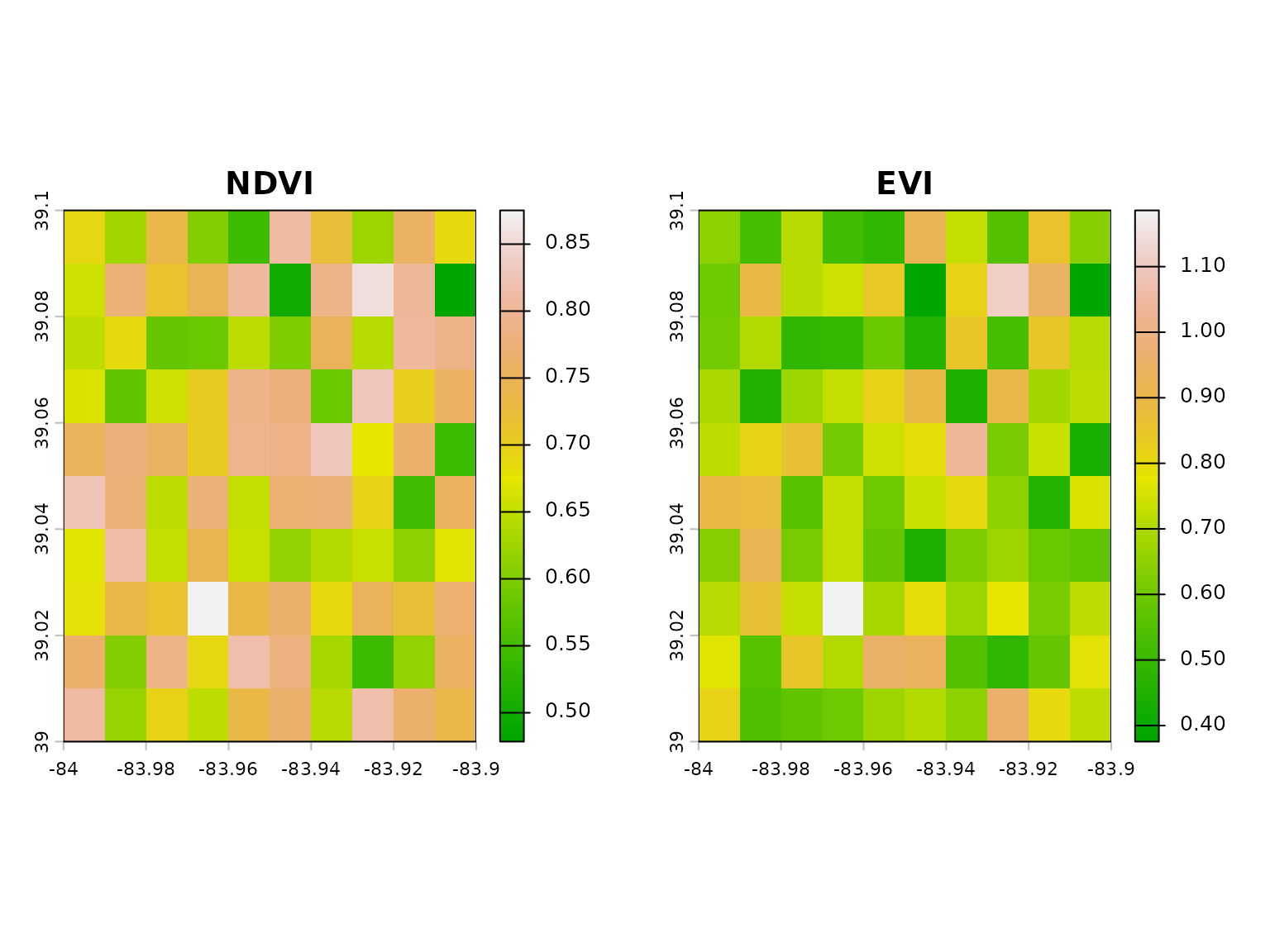

par(mfrow = c(1, 1))

SAVI (Soil Adjusted Vegetation Index)

# Calculate SAVI with geospatialsuite
savi <- calculate_vegetation_index(
  red = red,
  nir = nir,
  index_type = "SAVI"
)

plot(savi, main = "Soil Adjusted Vegetation Index (SAVI)",
     col = terrain.colors(100))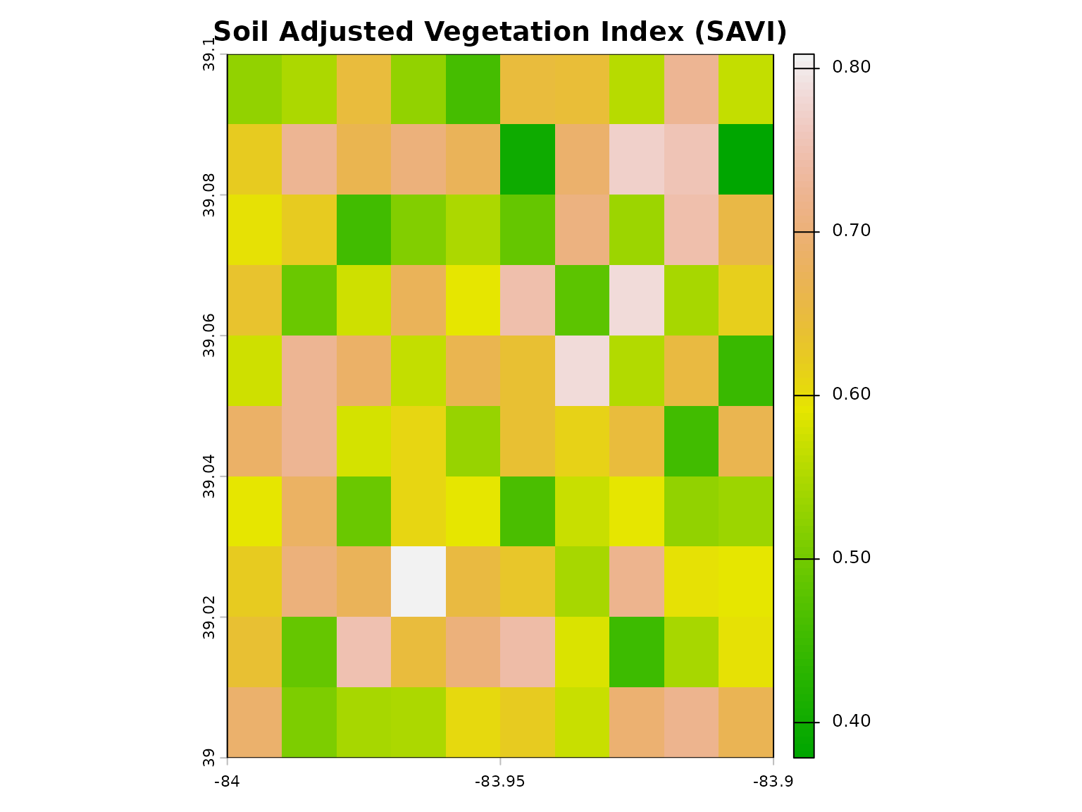

Calculate Multiple Indices

# geospatialsuite can calculate multiple indices at once
indices <- calculate_multiple_indices(
  red = red,
  nir = nir,
  blue = blue,
  indices = c("NDVI", "EVI", "SAVI", "GNDVI", "NDRE"),
  output_stack = TRUE
)

# Plot all indices
plot(indices, main = names(indices))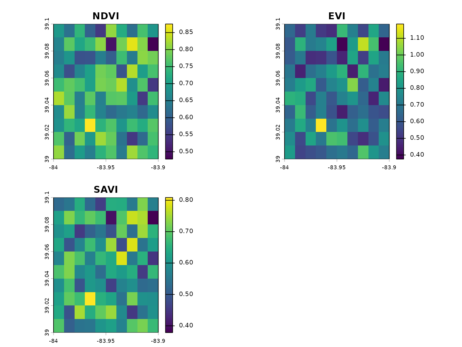


# Access individual indices
ndvi_layer <- indices$NDVI
evi_layer <- indices$EVI

Working with Multi-band Rasters

# Load multi-band raster
multiband <- load_sample_data("sample_multiband.rds")

# Check available bands
names(multiband)
#> [1] "blue"  "green" "red"   "nir"   "swir1"

# geospatialsuite's auto-detect feature
ndvi_auto <- calculate_vegetation_index(
  spectral_data = multiband,
  index_type = "NDVI",
  auto_detect_bands = TRUE  # Automatically finds red and nir!
)

# Calculate multiple indices with auto-detection
indices_auto <- calculate_multiple_indices(
  spectral_data = multiband,
  indices = c("NDVI", "EVI", "GNDVI"),
  auto_detect_bands = TRUE,
  output_stack = TRUE
)

Working with Satellite Imagery

Loading and Processing Landsat Data

# Use geospatialsuite with Landsat imagery

# 1. Load Landsat bands using geospatialsuite
landsat_bands <- load_raster_data(
  "landsat/LC08_L2SP_021033_20240715/",
  pattern = "SR_B[2-5].TIF$",
  verbose = TRUE
)

# geospatialsuite validates and loads all bands
# Extract individual bands (assuming they're scaled to 0-1)
blue <- landsat_bands[[1]]
green <- landsat_bands[[2]]
red <- landsat_bands[[3]]
nir <- landsat_bands[[4]]

# 2. Calculate indices using geospatialsuite
# It has 60+ pre-programmed indices
landsat_indices <- calculate_multiple_indices(
  red = red,
  nir = nir,
  blue = blue,
  green = green,
  indices = c("NDVI", "EVI", "SAVI", "GNDVI", "MSAVI", "OSAVI"),
  output_stack = TRUE
)

# 3. Visualize using geospatialsuite
quick_map(landsat_indices$NDVI, title = "Landsat 8 NDVI")

Processing Sentinel-2 Imagery

# Use geospatialsuite with Sentinel-2

# 1. Load Sentinel-2 bands using geospatialsuite
s2_bands <- load_raster_data(
  "sentinel2/S2A_MSIL2A_20240715/GRANULE/.../IMG_DATA/R10m/",
  pattern = "*_B0[2-8]_10m.jp2$",
  verbose = TRUE
)

# geospatialsuite handles JPEG2000 format
# Assuming bands are ordered: blue, green, red, nir
# and scaled to 0-1

# 2. Calculate comprehensive indices with geospatialsuite
s2_indices <- calculate_multiple_indices(
  red = s2_bands[[3]],
  nir = s2_bands[[4]],
  blue = s2_bands[[1]],
  green = s2_bands[[2]],
  indices = c("NDVI", "EVI", "SAVI", "GNDVI", "NDMI"),
  output_stack = TRUE
)

# 3. Visualize
quick_map(s2_indices$NDVI, title = "Sentinel-2 NDVI (10m)")

Multi-Temporal Analysis

# Track vegetation changes with geospatialsuite

# Load imagery from different dates
dates <- c("2024-05-01", "2024-06-01", "2024-07-01")
ndvi_series <- list()

for (date in dates) {
  # Load bands for each date using geospatialsuite
  bands <- load_raster_data(
    sprintf("satellite/%s/", date),
    pattern = "B[4-5].tif$"
  )
  
  red_date <- bands[[1]]
  nir_date <- bands[[2]]
  
  # Calculate NDVI using geospatialsuite
  ndvi_series[[date]] <- calculate_vegetation_index(
    red = red_date,
    nir = nir_date,
    index_type = "NDVI"
  )
}

# Stack time series
ndvi_stack <- rast(ndvi_series)
names(ndvi_stack) <- dates

# Visualize temporal progression
plot(ndvi_stack, main = paste("NDVI -", dates))

# Calculate change
ndvi_change <- ndvi_stack[[3]] - ndvi_stack[[1]]
plot(ndvi_change, 
     main = "NDVI Change (Jul - May)",
     col = colorRampPalette(c("red", "white", "green"))(100))

Specialized Vegetation Indices

Chlorophyll Content Indices

# Green NDVI - sensitive to chlorophyll content
green <- load_sample_data("sample_green.rds")

# Calculate using geospatialsuite
gndvi <- calculate_vegetation_index(
  green = green,
  nir = nir,
  index_type = "GNDVI"
)

plot(gndvi, main = "Green NDVI - Chlorophyll Indicator",
     col = colorRampPalette(c("white", "lightgreen", "darkgreen"))(100))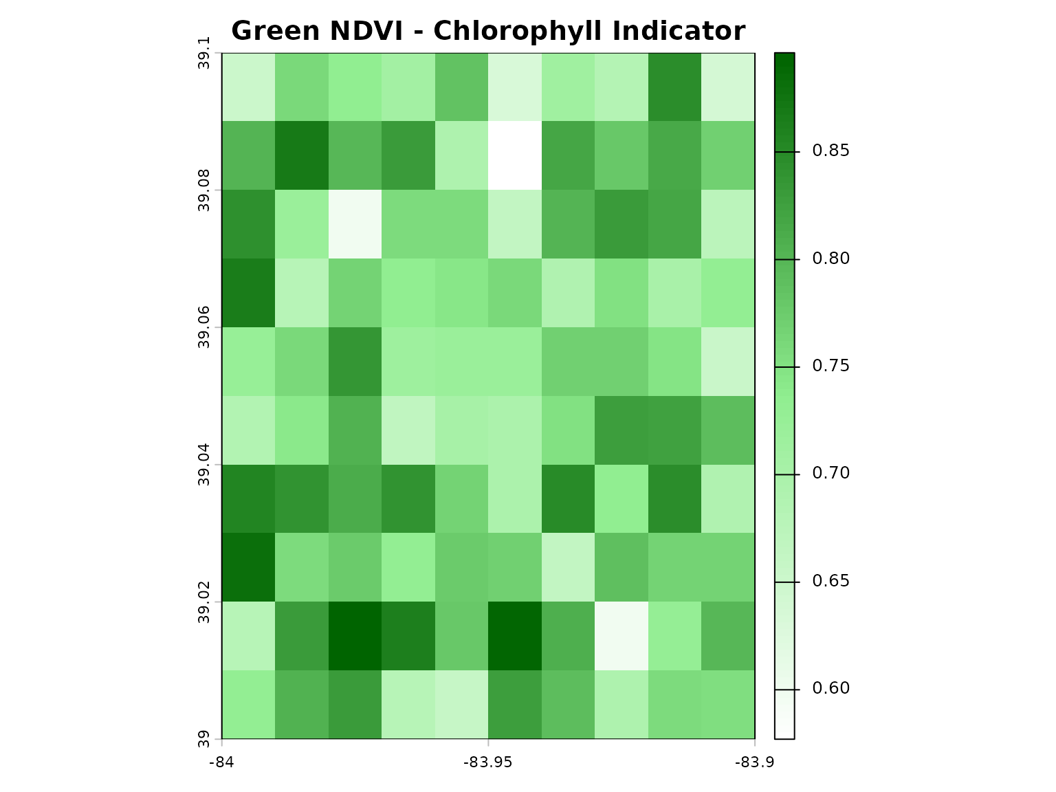

Water Content Indices

# Load SWIR band for water content analysis
swir1 <- load_sample_data("sample_swir1.rds")

# NDMI using geospatialsuite
ndmi <- calculate_vegetation_index(
  nir = nir,
  swir1 = swir1,
  index_type = "NDMI"
)

plot(ndmi, main = "Vegetation Water Content (NDMI)",
     col = colorRampPalette(c("brown", "yellow", "blue"))(100))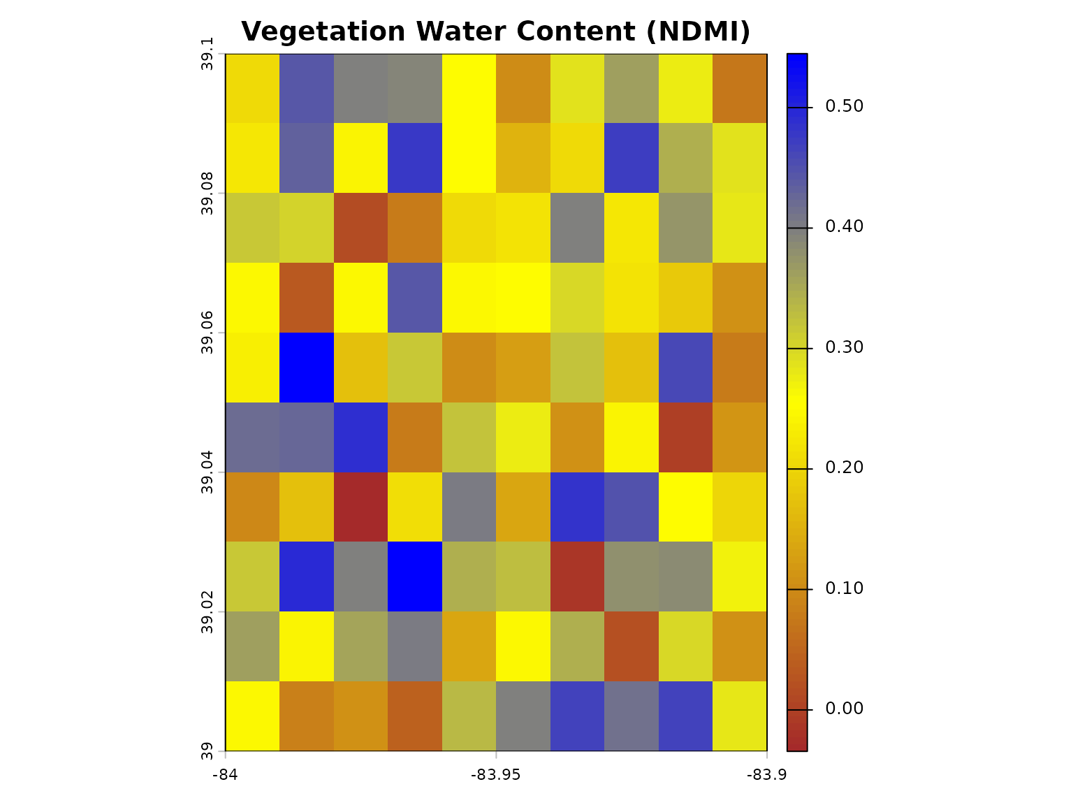

Advanced Analysis

Zonal Statistics

# Load sample boundary
boundary <- load_sample_data("sample_boundary.rds")

# Calculate NDVI using geospatialsuite
ndvi <- calculate_vegetation_index(red = red, nir = nir, index_type = "NDVI")

# Extract statistics for the region
stats <- terra::extract(ndvi, vect(boundary), fun = function(x) {
  c(mean = mean(x, na.rm = TRUE),
    sd = sd(x, na.rm = TRUE),
    min = min(x, na.rm = TRUE),
    max = max(x, na.rm = TRUE))
})

print(stats)
#>      ID     NDVI     NDVI.1    NDVI.2    NDVI.3
#> [1,]  1 0.706874 0.08445837 0.4784537 0.8752122

Field-Level Analysis

# Load sample field points
field_points <- load_sample_data("sample_points.rds")

# Calculate NDVI using geospatialsuite
ndvi <- calculate_vegetation_index(red = red, nir = nir, index_type = "NDVI")

# Extract using geospatialsuite's spatial join
field_ndvi <- universal_spatial_join(
  source_data = field_points,
  target_data = ndvi,
  method = "extract"
)

# View results
head(field_ndvi)
#> Simple feature collection with 6 features and 7 fields
#> Geometry type: POINT
#> Dimension:     XY
#> Bounding box:  xmin: -83.94662 ymin: 39.00987 xmax: -83.91607 ymax: 39.09223
#> Geodetic CRS:  WGS 84
#>   site_id  ndvi   evi crop_type elevation_m soil_moisture
#> 1 SITE_01 0.593 0.274  soybeans         269          0.27
#> 2 SITE_02 0.660 0.485     wheat         283          0.28
#> 3 SITE_03 0.646 0.579      corn         211          0.21
#> 4 SITE_04 0.388 0.483   pasture         256          0.31
#> 5 SITE_05 0.776 0.588      corn         219          0.35
#> 6 SITE_06 0.645 0.539  soybeans         205          0.30
#>                     geometry extracted_NDVI
#> 1 POINT (-83.94662 39.04604)      0.7709993
#> 2 POINT (-83.94162 39.00987)      0.7667765
#> 3 POINT (-83.94104 39.02066)      0.7647660
#> 4  POINT (-83.9309 39.09223)      0.7207893
#> 5 POINT (-83.93327 39.03194)      0.6405917
#> 6 POINT (-83.91607 39.02653)      0.7215534

Working with Real Field Data

# Complete field analysis workflow with geospatialsuite

library(sf)

# 1. Load field boundaries
fields <- sf::st_read("farm_data/field_boundaries.shp")

# 2. Load and process satellite data using geospatialsuite
satellite_bands <- load_raster_data(
  "satellite/imagery/",
  pattern = "B[2-5].tif$"
)

# 3. Calculate indices using geospatialsuite
indices <- calculate_multiple_indices(
  red = satellite_bands[[3]],
  nir = satellite_bands[[4]],
  blue = satellite_bands[[1]],
  green = satellite_bands[[2]],
  indices = c("NDVI", "EVI", "GNDVI", "SAVI"),
  output_stack = TRUE
)

# 4. Extract to fields using geospatialsuite
fields_with_indices <- universal_spatial_join(
  source_data = fields,
  target_data = indices,
  method = "extract"
)

# geospatialsuite extracted all 4 indices
# Each field now has mean NDVI, EVI, GNDVI, SAVI
names(fields_with_indices)

# 5. Visualize using geospatialsuite
quick_map(fields_with_indices, variable = "NDVI")

List Available Indices

# View all available vegetation indices in geospatialsuite
all_indices <- list_vegetation_indices()

# Show first few indices
head(all_indices[, c("Index", "Category", "Description", "Required_Bands")], 10)
#>    Index Category                              Description Required_Bands
#> 1   NDVI    basic   Normalized Difference Vegetation Index       Red, NIR
#> 2   SAVI    basic           Soil Adjusted Vegetation Index       Red, NIR
#> 3  MSAVI    basic  Modified Soil Adjusted Vegetation Index       Red, NIR
#> 4  OSAVI    basic Optimized Soil Adjusted Vegetation Index       Red, NIR
#> 5    EVI    basic                Enhanced Vegetation Index Red, NIR, Blue
#> 6   EVI2    basic       Two-band Enhanced Vegetation Index       Red, NIR
#> 7    DVI    basic              Difference Vegetation Index       Red, NIR
#> 8    RVI    basic                   Ratio Vegetation Index       Red, NIR
#> 9  GNDVI    basic                               Green NDVI     Green, NIR
#> 10  WDVI    basic     Weighted Difference Vegetation Index       Red, NIR

# Filter by category
health_indices <- all_indices[all_indices$Category == "basic", ]
print(health_indices[, c("Index", "Description")])
#>    Index                              Description
#> 1   NDVI   Normalized Difference Vegetation Index
#> 2   SAVI           Soil Adjusted Vegetation Index
#> 3  MSAVI  Modified Soil Adjusted Vegetation Index
#> 4  OSAVI Optimized Soil Adjusted Vegetation Index
#> 5    EVI                Enhanced Vegetation Index
#> 6   EVI2       Two-band Enhanced Vegetation Index
#> 7    DVI              Difference Vegetation Index
#> 8    RVI                   Ratio Vegetation Index
#> 9  GNDVI                               Green NDVI
#> 10  WDVI     Weighted Difference Vegetation Index

Best Practices

Index Selection Guidelines

NDVI: General vegetation monitoring
EVI: Dense vegetation, atmospheric correction
SAVI: Sparse vegetation, early growth
GNDVI: Chlorophyll content, nitrogen status
NDMI: Water stress detection

Data Quality Considerations

# Check for valid value ranges
ndvi <- calculate_vegetation_index(red = red, nir = nir, index_type = "NDVI")

# NDVI should be between -1 and 1
ndvi_stats <- global(ndvi, fun = "range", na.rm = TRUE)
cat("NDVI range:", ndvi_stats[1,1], "to", ndvi_stats[2,1], "\n")
#> NDVI range: 0.4784537 to NA

Summary

This vignette covered:

Using geospatialsuite’s calculate_vegetation_index() for 60+ indices
Using calculate_multiple_indices() for batch processing
Auto band detection with auto_detect_bands = TRUE
Loading satellite data with load_raster_data()
Spatial extraction with universal_spatial_join()
Multi-temporal analysis workflows
Field-level analysis
Best practices for index selection

geospatialsuite simplifies vegetation analysis with:

Pre-programmed indices
Automatic band detection
Robust error handling
Simple, consistent API

For more information:

Agricultural Applications with geospatialsuite
Complete Workflows and Case Studies
Getting Started with geospatialsuite

geospatialsuite Development Team